Quantcast
Channel: Dynamo BIM
Viewing all 41 articles
Browse latest View live

I love me a Parametric Bridge

$
0
0

I have a crap-ton of other stuff to do, and it’s sunny outside, but I know that you, dear reader, really really need  a slightly impractical bridge to get you into the weekend.  So here is my triumphant (and somewhat muttering) return to screencasting: setting out geometry for a fancy pedestrian bridge, from scratch, in Dynamo.

Download the .dyn file from here.

I will follow this up with clothing this in Revit structural framing, and flexing.


Improvements to Dynamo’s View Manipulation

$
0
0

Ever tried to rotate the background geometry preview but ended up showing a context menu for the nodes? Or tried to pan your graph but realized the geometry navigation is still active? Let’s face it, even the most active Dynamo user gets tripped up with these kinds of issues. If you’re like me, and you find this frustrating, you’re in for a treat.

In an effort to improve usability around view switching in Dynamo, we have made the following tweaks:

  • Added two in-canvas buttons to toggle between geometry and node views
  • Fade nodes out when geometry navigation is activated

In-canvas node and geometry switching buttons

There are now more ways than one to switch between geometry and node views, take your pick!

  • View menu > Background 3D Preview > Navigate Background 3D Preview
  • Shortcut CTRL + G
  • Hotkey Escape
  • “Geom” and “Node” buttons in the canvas

Now available on the latest daily build of Dynamo. Check it out if you’re living on the cutting edge and let us know what you think.

[Scratching the Surface of] Everything You Need To Know About Code Blocks

$
0
0

Simply put, Code Blocks are the bomb. If you’ve been following their development through the last six months of pull requests and Dynamo daily builds, you’ll know what I mean. There’s a lot going on in these little guys, and here is the CliffsNotes version of a how-to guide.

“Where did this come from!?” you ask. Dynamo and DesignScript, a text-based language for computational design, joined forces, and now there are more ways to make a series of points than I can count. And a lot of other stuff too.

It’s two good things in one. Like chocolate and peanut butter—chocobutter. Or if Brad Pitt and Angelina Jolie had a baby—that happened!

chocobutter

You too can make your own Code Blocks by double-clicking in the Dynamo canvas in version 0.7.0 or later.

Numbers, strings, and formulas

Code Blocks can hold numbers, strings, and formulas. You won’t even need those old-school nodes anymore. Enter a number like you would in the number node. Use quotation marks for strings. You can do any math in a Code Block that you could do in a Formula node. There are some differences, though; check out this post for a fuller comparison.

cbn01

All statements, or lines, in a Code Block must end with a semicolon. You’re allowed to be lazy for the last line you write; Dynamo will fill it in for you.

Calling other nodes

You can call any regular node in the library through a Code Block as long as the node isn’t a special “UI” node: those with a special user interface feature. For instance, you can call Circle.ByCenterPointRadius, but it wouldn’t make much sense to call a Watch 3D node.

Regular nodes (most of your library), generally come in three types:

    Create Create something
    Action Perform an action on something
    Query Get a property of something that already exists

You’ll find that your library is organized with these categories in mind. Methods, or nodes, of these three types are treated differently when invoked within a Code Block.

cbn12

Create.

When you use a method to create something, call it by name and specify the inputs in the order found in the out-of-the-box node.

cbn02

Create-type nodes that have no inputs still require parentheses.

cbn03

Action.

An action is something you do to an object of that type. Dynamo uses dot notation, common to many coding languages, to apply an action to a thing. Once you have the thing, type a dot then the name of the action. The action-type method’s input is placed in parentheses just like create-type methods, only you don’t have to specify the first input you see on the corresponding node since that’s the thing you are acting on, and you already know it.

cbn03

For example, if I want to call the node Point.Add from a Code Block, I notice that this is an action-type node. It’s inputs are (1) the point, and (2) the vector to add to it. In a Code Block, I’ve named the point (the thing) “pt”. To add a vector named “vec” to “pt,” I would write pt.Add(vec), or: thing, dot, action. The Add action only has one input, or all the inputs from the Point.Add node minus the first one. The first input for the Point.Add node is the point itself, which you already know or you wouldn’t be here.

Query.

Query-type methods get a property of an object. Since the object itself is the input, you don’t have to specify any inputs. No parentheses required.

cbn03

Flexibility

With Code Blocks, a user has flexibility to decide how to specify inputs. Here are several different ways to make the point (10, 5, 0).

cbn03

As you learn more of the available functions in the library, and you know what you want, you might even find that typing “Point.ByCoordinates” is faster than searching in the library and finding the proper node.

Make lists and get items from a list

Make lists with braces (a.k.a. “curly brackets”). Get items from a list with brackets (a.k.a. “square brackets”).

cbn03

Working with nested lists is just a variation on the theme.

cbn03

Replication guides

Replication guides set how several one-dimensional lists should be paired. It’s like list lacing but with more control. Use numbers in angle brackets with the inputs for a method. The hierarchy of the resulting nested list of results will be determined by the order of the numbers: <1>, <2>, <3>, etc.

In this example, I have lists of 2 x-values and 5 y-values. If I don’t use replication guides with these mismatched lists, I would get two points as a result, the same as the length of the shortest list. Using replication guides, I can find all of the possible combinations of 2 and 5 coordinates. And I can specify which list will be dominant: 2 lists of 5 things or 5 lists of 2 things. In the example, changing the order of the replication guides makes the result a list of rows of points or a list of columns of points in a grid.

cbn03

Make your own functions. Seriously.

Functions can be defined directly in a Code Block and called elsewhere in the Dynamo definition.

The first line has the key word “def”, then the function name, then the names of inputs in parentheses. Braces define the body of the function. Return a value with “return =”. Code Blocks that define a function do not have input or output ports because they are called from other Code Blocks.

Call the function with another Code Block in the same file by giving the name and the same number of arguments. It works just like the out-of-the-box nodes in your library.

cbn11

** This image was not altered! The Code Block on the right calls the function defined in the Code Block on the left. Same Dynamo file. “Look Mom, no wires!”

04_CodeBlockNodes

Find these and other examples in CodeBlocksForDummies.dyn.

Math Transit

$
0
0

With the arrival of Code Blocks in Dynamo version 0.7.0 and later, there are now at least four distinct options for calculating stuff:

  1. Traditional nodes
  2. The Formula node
  3. Python
  4. Code Blocks

(There’s a fifth method, too, if you write your own node, compile it, and import the dll using zero-touch import—look for a future blog post!) And any of these methods could be wrapped in a custom node. The point is, there’s now a lot going on in Dynamo. This blog post is meant to serve as a Rosetta Stone: how to calculate stuff different ways.

For purposes of making the comparison clear, I’ve chosen to generate the same cool surface from a grid of points whose z-coordinate I will spend the rest of this blog entry calculating. The surface is a solution to this equation (A and c are constants):

eqn

Traditional nodes

Pros Cons
  • No special syntax to know
  • Can check data at intermediate steps
  • Hard to decode later
  • Logic not visually obvious
  • Lots of mouse clicks
  • Inputs not clearly labeled

math01

With this and other example images in this post, click the image to see the full graph that makes the surface. Download the .dyn file with all four examples at the bottom.

Everybody loves using traditional nodes. But using them may not always be the best solution. The image above shows one possible arrangement of traditional nodes that solves the surface equation. The graph might look familiar and comfortable to the person who made it, but it might not be obvious to others what it does unless it’s well-labeled. Having clear logic in your graph helps your future-self and coworkers decode what your present-self was thinking. This is especially true when dealing with math-heavy operations, when there is no geometry to preview to help you figure out what’s going on.

Dynamo version 0.7.0 and later uses degrees for angles. You may note the use of the node Math.RadiansToDegrees because formulas such as this expect angles in radians.

Formula node

Pros Cons
  • Inputs are clearly labeled
  • Similar syntax to a graphing calculator
  • Easy to edit
  • Concise
  • Everything must be written in one line
  • Hard to check data at intermediate steps
  • Expects angles in radians

math02_close

For more information on the Formula node and its syntax, see the post NCalc and Dynamo’s Formula node. The Formula node has clear advantages for working with math-heavy operations, and its syntax will be familiar to anyone who has ever used a graphing scientific calculator.

The Formula node, which uses an external library of functions, expects angles in radians. Documentation for the NCalc project‘s syntax can be found at:

Python

Pros Cons
  • Can use Python if you know it
  • Can use loops
  • Concise
  • Inputs not clearly labeled
  • Have to know Python
  • Lots of boiler-plate code required
  • Must be specific when dealing with single items vs. lists
  • Not as easy for co-workers to edit
  • Hard to check data at intermediate steps
  • No one is holding your hand

math03

Python is a powerful tool, relatively unlimited in its capabilities. But you have to know Python. And burying your code in a Python node is as close to making a “black box,” where everything is obscured, as you can get. Check out this blog post for more information on the Python node.

Double-click a Python node to see its innards. Inside this one, you’ll see:

math_python

You’ll notice some boiler-plate text at the top, which is meant to help you reference the libraries you’ll need. To the standard text, I’ve added a statement to import the math library. Inputs are stored in the IN array. When extracting the inputs from IN, I just have to keep track of the order in which I attached the inputs. Values are returned to Dynamo by assigning them to the OUT variable.

To solve the equation for a grid of points, I will have just one value for the constant amp and one value for the constant c, but I will have a potentially long list of x- and y-values. With Python, which operates outside the cozy context of Dynamo, you will have to be explicit about what you’re working with: single-values or lists of values. I’ve used a for loop to parse through the list of x-values, finding one new z-value for each. The code I’ve written is less robust than the three other methods. I have assumed, for instance, that I will have at least as many y-values as x-values. And I’ve assumed that amp and c inputs will be single values. The code might break and return an unfriendly error message rather than a nice list of z-values if my co-worker hooks up the inputs wrong. There is no automatic lacing here like in Dynamo. Of course, you can make this Python code just as robust as anything else by adding in checks or by generalizing the logic that solves the equation, but I will leave that as an exercise for the reader. My point is: no one is holding your hand in Python land. For solving math problems, there are usually better ways.

Code Blocks

Pros Cons
  • Flexible formatting
  • Easily check data at intermediate steps
  • Inputs are clearly labeled
  • No boiler-plate code necessary
  • Concise
  • Easy to edit
  • “The world is your oyster.”

math04

Code Blocks are magic. And in case you haven’t noticed yet, I have a clear bias toward them. Especially for math. Note that I have used the function Math.RadiansToDegrees() just as I had to for the traditional nodes solution because Dynamo expects angles in degrees.

With a Code Block, you can call any other node in Dynamo. Imagine all of the advantages of the traditional node-based method together with a clear, concise, easy-to-understand and easy to change block. Read more in the post [Scratching the Surface of] Everything You Need To Know About Code Blocks.

For a moment, forget how you would solve this with nodes, calculators, or code. If your teacher assigned this problem as homework and you had to work out the answer on paper, how would you do it? Here’s the problem:

math_1

I’ve graded enough homework assignments to know that there are an infinite number of ways to solve even the simplest problem, and some are even correct. Among the myriad possibilities, here’s one.

math_2

Notice that I’ve structured my solution with a Code Block the same way. And when you change your single x- and y-value to a series of points, it just works. If you handed me your Dynamo definition and asked me to fix something, I would much rather try to figure out what you did if I could read Code Blocks!

For kicks, check out the similarity between the Python code—specifically the part that matters—and the Code Block.

compare

Code Blocks give you a lot of the power of Python without all the other stuff.

So, which method do you like best? Download the sample file MathTransit.dyn.

mathExample

Making it real

Once I have a surface in Dynamo, I can use it as a scaffolding to place panels in Revit.

remapAndColor

With this logic tacked on to the end of the surface, I use a custom node from the Package Manager called UV Quads on Surface to create a grid and organize points into groups of 4 describing each cell in the grid. I use those points to place an adaptive component. I use a reporting parameter in the adaptive components that describes the amount of deflection—by how much the panel is out-of-plane—and I use those numbers to pick from a color range from blue to red. Then I use that information to color the components, in Revit, according to their planarity.

colorInRevit

INTERSECTING RAILS

$
0
0

The Dynamo blog is pleased to welcome this guest post by Eduardo Perez Roca. Eduardo is a regular contributor to the Dynamo community and forum. He is a senior architect specialized in the development of complex geometries in a well known international office.

Intersecting_Rails_01

A new kind of tool was introduced between 2008 – 2010. Tools like Revit Adaptative Components, Inventor ICopy and CATIA PowerCopy. All of them allow the same prototypical workflow: driving “flexible” components with points resulting from the intersection of curves (“rails”) with an array of planes.

I have used both Revit and Inventor tools extensively since 2010. With these tools, going from the nice and simple demonstration tests to large and complex projects with hundreds or thousands of different elements is quite a challenge.

The typical issue

Intersecting_Rails_02

All these tools will work smoothly as long as the rails are nice, continuous curves. Depending on your choice of tool, you might be able to manage using joined curves as a rail, even with sharp corners. But any gap or overlap will be a problem. For small gaps, sometimes it is possible to remap a group of curves in a single curve, “jumping” over the gaps. But any big gap, or big overlap, and you can forget about it.

In real projects, gaps, overlaps and sharp corners are quite common, so the standard toolset will not allow for a one-size-fits-all solution. You must deal with this problem by dividing the project in smaller parts, where the rails will be “good enough.”

The solution

The new Dynamo allows us to move past this issue. And the solution is just a few lines of DesignScript.

Intersecting_Rails_03

The way of managing this is quite simple using DS code, which is extremely efficient for geometrical operations. Instead of choosing which plane to intersect with which curve, each single plane is intersected with all the curves. A smart, built-in function deals easily with the case of no intersection. If more than one intersection is found (overlapping lines), only one point is taken.

We can get the intersection points for any group of curves in the same way we would for any simple curve. And without trying to join the curves or build a new, single curve equivalent to the original group.

RailsIntersection

Intersecting_Rails_04

This solution is implemented in the custom node RailsIntersection, which can be seen here and found in the middle of the workspace at the beginning of this post. It includes some additional functionality in order to filter and organize the groups of points. You can find it in the package manager.

The value passed to the input “N Points” sets the expected number of points to be returned when intersections are found for more than one rail. The value of N will mean that you want sets of at least N points

Intersecting_Rails_05

Intersecting_Rails_06

Pass in a value of zero to find a result for every plane, including en empty list each time a plane finds no intersection.

The custom node expects that every rail is a list of objects. If you will use for rails that are just a single object (one curve or one polycurve), that single object must be inside of a list.

Not just points

Beyond points, Dynamo 0.7 allows us to directly create the solid (or surface) geometry of the final components with its own modeling tools. Dynamo now provides access to the same geometry engine as Inventor, the Autodesk Shape Manager (ASM). Just as in previous versions of Dynamo, you can use the points for driving Revit Adaptative Components (and maybe Inventor ICopys or something similar in a not so distant future).

Choosing whether to place adaptive components or to model the geometry with algorithmic logic is a matter of convenience (whether it makes sense). For typical “frames,”using Dynamo’s own modeling tools is far more practical.

Intersecting_Rails_07

This sample includes components of one, two and three segments. With Adaptative Components (or similar tools), three different components would have to be defined and placed. With Dynamo’s geometry tools, this is the same sweep operation along several curves. Besides of this, the way of managing the profiles (to change them or add several ones) is more straightforward and easier.

Intersecting_Rails_08

And Dynamo is a more convenient platform to add complexity to the paths like curved segments. In the sample, two DS functions are used for controlling when and how the last segment is curved. A simple rule is set for using normal arcs where possible and NURBS curves when arcs would not match the design intention. The result, in this case, is that half of the curved segments are normal arcs.

Using the “pre-release”

After the 0.7.0 “pre-release”, I rebuilt an old ICopy development in Dynamo, which had roughly a thousand different elements. I used the standalone version, importing the context geometry and the profiles from Inventor. And my experience was extremely positive.

There is a big boost in performance. The times for updating have gone literally from minutes to seconds. For the first time it is possible to make quick design iterations, fully updating large models. Another big difference is greater “parametric robustness”. There is no need to fix or rebuild anything after changing all the driving lines. And by change, I mean fully deleting and creating new curves, not just flexing the existing curves.

Taking into account the state of development, with probably a few enhancements to come, Dynamo looks like an impressive platform for this kind of workflow.

Cleanup Node Layout

$
0
0

Be honest, does your graph ever look like this?

hairball

New in Dynamo v0.7.1, Cleanup Node Layout. Accessed in the Edit Menu or with the shortcut CTRL+L.

cleaner

In this post, I present the great work of Ellensi Chandra, who recently completed a 6-month internship with the Dynamo team in Singapore. At the end of May, developers on the Dynamo team took two weeks to pursue whatever project they wanted for Dynamo, for a time setting aside the normal crush of development tasks. We called it a “recharge” after the successful completion of the migration tasks to make sure all of your v0.6.3 files will translate as best as possible to the new v0.7.1. This was Ellensi’s project.

They say “there’s more than one way to skin a cat.” (Sorry Snowball II!) Here are some of the many ways to lay out a graph.

cleanup00

Any takers on implementing the circular layout algorithm!? For visual scripting, some of these are clearly more useful than others. Dynamo’s new automatic graph cleaner-upper is a version of a layered diagram. Dynamo’s algorithm:

  • Is fast
  • Enforces a left-to-right data flow
  • Organizes input nodes on the left and output nodes on the right
  • Preserves the top-to-bottom order of output nodes (blue, yellow, then red below)

cleanup10

  • Distributes nodes evenly
  • Keeps Wires as straight as possible
  • Minimizes the number of wire crossings (18 crossings becomes just 3 below)

cleanup11

Try it out on your graph with CTRL+L or find it in the Edit menu. Undo is implemented too, so if you don’t like it, type CTRL+Z to revert to what you had before. It’s fun. But it’s probably not the perfect solution for everyone yet. Current limitations are that it operates on the whole graph, not just a section, and notes are not yet included with the reorganization. Still, it’s an exciting direction for Dynamo.

How?

Graph theory (which is surprisingly useful, far, far beyond visual scripting) is the study of networks of paired pieces of information. Your GPS device uses graph theory techniques to find the best route home from a party. And, if you were so inclined, you can use graph theory to prove that you only need 4 colors to color any map without having any country/state touching any other state with the same color.

colorMap

        Images from http://world.mathigon.org/Graph_Theory.

Your Dynamo graph is, in fact, a graph. Hence the name. If we use official terminology, your nodes are vertices and your wires are edges. Edges are a record of which vertices are paired to which other vertices. And edges can be directed, or “pointing” in one direction. The wires in your Dynamo graph are directed because information only flows one way through them, from some output port to some other node’s input port.

The automatic layout algorithm uses these relationships to reorganize the nodes and wires. Dynamo’s algorithm is a version of the Sugiyama Method for organizing a graph, which has four steps.

Step 1: Cycle Removal A cycle is a lot like what it sounds like. Following the data flow from one node, you should not be able to get back to that same node. If a node is dependent on its own output, you have a condition known as a circular reference, which Dynamo doesn’t support. And it doesn’t make any sense any way.

cleanup01

        Diagram series from http://sydney.edu.au/engineering/it/~shhong/fab.pdf.

Step 2: Layering For Dynamo’s implementation, this means assigning nodes to columns. Input nodes, or those that don’t have any dependencies (sliders, number nodes, file paths, etc.) are all assigned to the first column. Output nodes, or those that don’t pass any information to anything else go to the last column. The rest is kind of magic. I’ll let you read about it here: Coffman-Graham algorithm.

cleanup02

Step 3: Node Ordering Once nodes are assigned to columns, next Dynamo finds the vertical order of the nodes that creates the fewest number of wire crossings. The Dynamo implementation starts with the order of the output nodes and works backwards, arranging the columns of upstream nodes, to untangle them using the Median method.

cleanup03

Step 4: Coordinate Assignment This step, unique to the Dynamo implementation, assigns coordinates to the nodes including considerations for the order of the input ports on each node.

cleanup04

Enough said:

snowballHappy

Dynamo 0.7.1 Release

$
0
0

2014-06-26_2243

Dynamo version 0.7.1 officially replaces version 0.6.3 as the most recent stable build. The shift from Dynamo 0.6 to 0.7 represents a significant refactoring of the original code base. The new software architecture allows for better performance, more robust geometry, sophisticated interactions between traditional scripting and visual programming, and loading of external software libraries. If you followed along with the development process over the past few months with the daily builds and the 0.7.0 alpha release, you’ll know that there is a lot that’s new. We hope you’ll love it.

New in Dynamo 0.7.1:

  • Revit 2014 and Revit 2015 compatible
  • Dynamo runs standalone, without Revit
  • Integrated DesignScript syntax in code blocks (See the blog post.)
  • Vastly expanded geometry library (See the blog post.)
  • Automated upgrading from 0.6.3 files to 0.7
  • Visualization performance improvements
  • Library reorganization
  • Library loading (experimental)
  • New opening page
  • Node UI enhancements
  • Node/Geometry navigation improvements (See the blog post.)
  • Automated graph organization (See the blog post.)
  • Preview Bubble overhaul
  • New sample content
  • New file structure (See the blog post.)

The last alpha release, version 0.7.0, was the initial release to demonstrate some of Dynamo’s new capabilities. Since then, we have been improving stability and building an automated migration manager to preserve as much of your 0.6.3 workflows as possible. Find more info at the Dynamo Wiki. Stay tuned for a blog post on migrating your workflows from 0.6.3 to 0.7.1.

Geometry

The new geometry tools in Dynamo 0.7 are vastly expanded from those that were available in 0.6.3 and earlier versions. Dynamo now has the same geometry engine that supports Inventor, Fusion, and other Autodesk products. No longer is Dynamo—or Revit—limited to the geometry available from Revit’s conceptual mass editor.

In the words of Peter Boyer, Dynamo developer: “Revit, meet NURBS.”

revitNurbs

Rather than give you a catalog of everything the Dynamo geometry library allows you to do, you should check it out yourself. There are now fully five ways to make a circle. I rest my case.

fiveCircles

Download the sample file FiveCircles.dyn.

Code Blocks

Code blocks will change your life. They’re awesome. The release of Dynamo version 0.7.1 marks the end of the first step in integrating the text-based language DesignScript into Dynamo’s visual scripting environment, which provides a powerful alternative to and extension of node-based scripting. But don’t worry—nodes are not going away! Code blocks simply let you script faster and more precisely with the same language of nodes, inputs, and outputs that you’re used to in the rest of Dynamo. There is so much to say about code blocks:

Here’s how to use them:

Here’s why to use them:

Code blocks give you flexibility. They can hold numbers, formulas, strings, and call any other node! Now there are even more ways to get your work done. Here are four different ways to make the same point:

cbn06

All-new sample files

newSamples

The best way to learn is by doing. Check out the new collection of sample files, which install with Dynamo, and can be found in the help menu. Samples are organized in five categories:

Basics Visual scripting, points, and creating series
Core Advanced lists, code blocks, functions, and strings
Geometry Curves, surfaces, and solids
Import/Export Moving data to and from CSV and Excel
Revit Adaptive families, color, floors, and levels

When you install Dynamo, the sample files are written to C:\ProgramData\Dynamo\0.7\samples. This is a hidden folder in Windows, so to get there, you will either have to view hidden folders or type the address directly into the search bar. All of the Revit samples are made to work with one base file: C:\ProgramData\Dynamo\0.7\samples\Revit\DynamoSample.rvt. To run these samples most effectively, open this Revit file first, then open the sample file in Dynamo.

User experience improvements

New start page. Easily access recent files, examples, learning materials, the forum, and more.

frontPage

Gray is the new orange. You spoke, we listened.

orangegray

Library reorganization. Each section of the library is generally organized with the subcategories Action, Create, and Query. The Create category contains nodes that create objects of that type, like making a circle from a point and a radius. The Action category has nodes that do something to an object of that type, like chopping a list in pieces. And the Query category contains nodes that you extract information that already exists, like getting a parameter value from a Revit element.

cbn12

New node naming convention. “Normal nodes,” most of them, now have a two-part name separated by a dot that tells you (object).(what it does). They’re like small sentences. List.Create makes a list. Circle.ByCenterPointRadius makes a circle using a center point and a radius. You get the picture. Anything starting with “By” like ByCenterPointRadius or ByCoordinates makes something. Operators like add, greater than or equal, and multiply are named simply by the symbol you would use when you type them: +, >=, *, etc. Built-in functions (there’s a special category for them) and other “UI”-type nodes like Watch and Slider do not use the dot notation (they aren’t callable from code blocks).

nodeNames

Automatic graph organization. This could be useful to clean up migrated version 0.6.3 workflows that look cluttered. See the blog post here.

cleaner

Visualization performance enhancements. Besides being faster, you now have direct control over the precision with which your geometry is rendered. With large, highly curved models, you may want to turn down the precision for faster interaction. Turn it up (in the Settings menu) to see your curvy creations more accurately.

renderPrecision

Geometry view. New visualization ability with “Geom View” to navigate the background preview without so many nodes in the way. Toggle between “Geom View” and “Node View” with the buttons in the canvas, the option in the View Menu, the shortcut CTRL+G, or the Escape hotkey. See the blog post here.

geommode

Where Does My Dynamo Live?

$
0
0

DynamoHome

Your Dynamo has moved. And it has moved up in the world too, from the starter home on your C-drive to a new estate, with room to grow, in the up and coming Program Files neighborhood. This post will help you understand where your Dynamo files are and what they do.

smallFolder

Program Files

C:\Program Files\Dynamo 0.7

As of version 0.7.1, Dynamo installs to your Program Files directory, following Windows guidelines. Subsequent releases in the 0.7-branch will install in \Dynamo 0.7, while future releases in the 0.8-branch will live next door in \Dynamo 0.8 and so on. This will allow you have multiple versions of Dynamo available at once time when there are substantive updates.

Inside C:\Program Files\Dynamo 0.7 are folders for each supported version of Revit, currently Revit 2014 and Revit 2015. All top-level files here are for Dynamo’s core functionality, used for both standalone and Revit Addin modes. Changes to files in this directory require administrative permissions, and users should never need to change these files.

You will find the executable file for the Dynamo standalone version here, called DynamoSandbox.exe. For easy future access, place a shortcut on your desktop. Find this file, right-click on it, and choose Send toDesktop (create shortcut).

standaloneLocation

smallFolder

ProgramData

C:\ProgramData\Dynamo\0.7

Any data that comes installed with Dynamo that is not specific to the user is stored here. ProgramData is a hidden folder in Windows, so to get here, you will have to show hidden files or type the address directly into the address bar. Inside you’ll find a folder containing the sample files available from the Help Menu and a set of definitions (custom node files with a .dyf extension) that help support migrated version 0.6.3 workflows.

Files in this location are available to all users on the local machine, and administrative permissions are not required to make changes.

samplesfolder

smallFolder

AppData

C:\Users\your_name\AppData\Roaming\Dynamo\0.7

Any data specific to a user is stored in the AppData folder, which is also a hidden folder. Here you will find folders for log files, definitions (custom node files) and packages that are specific to a user. Beginning users should not have to touch files in this folder, but the option is available for users who want to manually move definitions and packages between user accounts.

Dynamo uses \AppData\Roaming, as opposed to \AppData\Local, so that these files will follow the user’s credentials around an office network. Now when you download a package to your library at your desk machine, you will also have them available when you log into any other computer on the network. Some office networks have custom settings that could interfere with this behavior.

Administrative permissions are not required to make changes in this location. When new Dynamo installers run, they will not delete or alter the user’s definitions and packages folder.

smallFolder

Addins

C:\ProgramData\Autodesk\Revit\Addins\2014
C:\ProgramData\Autodesk\Revit\Addins\2015
C:\ProgramData\Autodesk\Vasari\Addins\2014

When the Dynamo installer runs, you have the option to install an addin for any of the versions of Revit that are supported and available on your machine. The installer looks for which versions of Dynamo you already have installed (for example, an earlier version), and it will generate and place the appropriate addin files in the appropriate folders. The addin files in the locations listed above point to the appropriate version of the Version Selector addin, which allows you to select which version of Dynamo you want to use.

To clarify, the Version Selector is a second Revit addin, in addition to Dynamo itself, that registers the “old” version of Dynamo (0.6.3) and the new version of Dynamo (0.7.x) and provides a button in Revit to allow you to switch between these. (It’s the best solution available within the context of the Revit Ribbon to allow you to have more than one Dynamo version installed.) You should never have to touch these files, but it may help you to know they’re there.

versionSelector

smallFolder

Moving In…

Some advice to help you move your older files to their new locations. Your old files at C:\Autodesk\Dynamo\Core and C:\Autodesk\Dynamo07\Core are no longer needed once you switch over fully to version 0.7.1. The installer for 0.7.1 will clean up the core files for the Dynamo 0.7 branch but will leave your definitions and packages folders so that you can bring them over to their new home in AppData when you’re ready.

To move your files, just select them from the definitions or packages folder at C:\Autodesk\Dynamo\Core and paste in the definitions or packages folder at C:\Users\your_name\AppData\Roaming\Dynamo\0.7\definitions. Then you can delete your Dynamo folders from C:\Autodesk. You’ll want to make sure that your old files work as expected in the new version.


Geometry 101

$
0
0

Dynamo’s new geometry library, as of the 0.7 branch, vastly expands your capability to model complex forms both in Dynamo and in any platform it touches. Can you imagine modeling a woven basket in Revit? Well, now you can. There is more to tell than can fit in any one blog post, so to learn more about any of these projects, get your hands dirty and download the sample file at the end of each section. Each of the projects is fully parametric, and you will be able to follow changes in an input slider through each graph by previewing geometry and looking at Watch nodes. Feel free to discover faster, more efficient, or more intuitive ways to solve some of these problems than I found.

Why are we modeling three different baskets? Because it’s a good scale to work with, and everyone likes a theme. We’ll call this one: Basket Case.

Special thanks to 360 Architects in Kansas City for the genesis of the idea for basket #1. It came out of a fun collaborative workshop session where we were exploring the then-brand-new geometry tools of Dynamo 0.7.0.

01. Solid Booleans and Transformations

basket1Variations

This complexity of this “basket,” if you can call it that, lies in rotational transformations of rings. The rings themselves are made from the Boolean difference of two solid disks. Solid Boolean operations are particularly fast in Dynamo, especially as compared to Revit.

basket1_01 Array points equally around a circle. Use a series of parameters from 0 to 1 and Curve.PointAtParameter. Remember to account for the fact that the start and end points will be the same for a closed curve.
basket1_02 Draw larger circles around each of these points.
basket1_03 Extrude larger circles and slightly smaller circles just inside these with Curve.ExtrudeAsSolid. Use Solid.Difference to subtract the solid of the smaller disc from the larger disk, leaving a hoop.
basket1_04 Rotate each hoop about the radius of the small circle in the middle with Geometry.Rotate.
basket1_05 Rotate each hoop a second time about the tangent of the small circle.
basket1_06 Increase the number of hoops.

basket1File

Download the file: Basket1.dyn.

02. Points, PolyCurves, and Extrusion

basket2Variations

Points and lines are fundamental building blocks for most geometric projects in the scripting world, and this example makes good use of points in particular. Note that it is sometimes more convenient to treat points as vectors and that much of the geometric logic lies in the order of points in a list.

(The form of this basket is sometimes called a scroll saw basket. It’s made by sawing a flat piece of wood into a spiral, and the walls can be brought up from the base like a coiled spring.)

basket2_01 Rotate the Vector.XAxis to the appropriate angles (360°/#sides) with Vector.Rotate. Scale each of these radial vectors with a series. Treat the inside of the spiral and the outside of the spiral separately. Create points from the vectors with Vector.AsPoint.
basket2_02 Rearrange the list of points so that they are organized in rings, then Flatten the lists into a spiral. Add a series of incrementally increasing vectors in the z-direction to the points with Point.Add to move them up.
basket2_03 Reorganize the points into sets of four with List.Sublists, List.Reverse, and List.Join to describe the corners of each spiral segment. Create closed polycurves from these with PolyCurve.ByPoints.
basket2_04 Create a solid for each segment with Curve.ExtrudeAsSolid. Optionally, join all of the solids together with Solid.UnionAll.

basket2File

Download the file: Basket2.dyn.

03. Intersection, Loft, Sweep, and Thicken

basket3Variations

No lineup of baskets would be complete without something woven. And though weaving is perhaps more a demonstration of advanced list manipulation logic than strict geometry, this particular example shows off the power of NURBS curves, lofting, and surface thickening tools in Dynamo. You’ll definitely want to download this file, below.

basket3_01 Create two ellipses and a point at the bottom that will define the shape of the basket. Use any shape you like. Your life will be simpler if the point at the bottom is Point.Origin.
basket3_02 Array a number of planes evenly between 0° and 180° at the center. Find the intersection points between each plane and the ellipses with Geometry.Interesect.
basket3_03 Use these points to define planar NurbsCurve.ByPoints‘s that will be the scaffolding for the “staves,” or “spokes,” of the basket.
basket3_04 Use Curve.PointAtParameter to find the points where the weaves will cross. Draw line segments tangent to the curves there with Curve.TangentAtParameter and offset these toward the inside and outside of the basket.
(See Vectors, below.)
basket3_05 With a little bit of list logic, connect the end points of every other line inside the basket with every other line outside the basket. You’ll need two opposite sets of curves for each weave to choose between later.
basket3_06 Create a Surface.ByLoft between the top and bottom NURBS curves. Make the surface into a solid with Surface.Thicken.
basket3_08 Cut off the construction lines at Geometry.GetClosestPoint for each of the staves with the top of the top weave. Draw lines at one end of each stave line perpendicular to the plane of the curve. (See Vectors, below.)
basket3_09 Sweep the lines into surfaces with Surface.BySweep and thicken these surfaces as before.

basket3File

Download the file: Basket3.dyn.

04. Vectors

In scripted geometry, vectors are king. A vector, of course, is just a direction and a magnitude—an arrow, if you will. But there is so much hidden power to be harnessed to bend parametric surface to your will!

In this example, I simply explain how I calculated the vectors for basket #3 that pointed inside and outside the basket, perpendicular to the construction curves, at each point where a horizontal weave crossed a vertical stave. Once I had these vectors, they were immensely valuable throughout the rest of the definition.

VectorDiagram1

First, pick a point along the curve with Curve.PointAtParameter.

VectorDiagram2

The vector parallel to the curve at that point is called the tangent, and you can find that directly too with Curve.TangentAtParameter.

The task remains to find a vector that is perpendicular to this one, but pointing either directly outside or inside the basket. The problem is that there are an infinite number of vectors perpendicular to this tangent vector, and to choose just one, we have to apply the restriction that it lie in the plane of the construction curve.

VectorDiagram3

One trick, is to find any other vector (not parallel to the first vector) in the plane of the construction curve. Since all of the construction curves run through the origin, a vector from the origin, to that original point will do the trick. For insurance, to make sure the new vector won’t line up with the tangent vector, I’ve also made the new vector from the origin parallel to the horizontal, XY plane.

VectorDiagram4

Once I have two vectors in the plane of the construction curve, I can take their cross product with Vector.Cross to get a vector that is perpendicular to both of the original two vectors. This is the same as the normal of the plane containing the blue construction curve.

(This might sound complicated, and you could find the plane of the curve first and just take the normal instead, but look how few nodes it takes to use vectors directly!)

VectorDiagram5

I can then use just one more cross product operation to find the vector that is perpendicular to both the tangent vector (red) and the side-to-side vector (teal) to give me the final offset vector (green), which is the vector pointing outside the basket. The vector pointing inside is simply the negative of this one, or Vector.Reverse.

05. Make it Real

Okay, so how does any of this make it into Revit? Potentially a lot of ways—you can use geometry in Dynamo as a scaffolding to place Revit Elements, or you can import an instance of the geometry directly into a Revit family or project. For that last method, you have two options for this, ImportInstance.ByGeometry, which imports each item in a list as separate Revit imports, or ImportInstance.ByGeometries, which imports a collection of geometries, all at once, into one selectable Revit import instance.

importInstance

Design alternative for the Sony Center in Berlin… ? Anyone… ?

newSonyCenter

Image of Sony Center from here.

RGB Transform

$
0
0

Transform_02

Red for the X axis, green for the Y axis and blue for the Z axis. Like many other software with 3D environments, Dynamo uses the known order of basic colors to help to differentiate the axes of the coordinate systems.

In my previous post “Intersecting rails”, it was implicit the potential of Dynamo to automatically replicate and reposition profiles. This is a previous step when making multiple elements at once via sweep or loft. This post goes into the details about how to achieve this and some practical related issues.

Copy + align + ……. = Transform

Geometry.Transform is one of the core methods of Dynamo. It replicates any geometry from one coordinate system to another. The initial and the resulting geometry maintain the same position relative to their coordinate systems.

One habitual use of transform is combined with the methods that return coordinate systems (C.S.) aligned with curves and surfaces. It allows copying directly any geometry following curves or surfaces. In the case of making sweeps, CoordinateSystem.AtParameter (or AtDistance) gives us the C.S. aligned with the paths.

Transform_12

The default axis configuration maybe is not going to match directly what we need. In the sample above the profile is done in the plane XY. So we need the new X and Y axis to be perpendicular to the path. But the default C.S. aligned with the curve are having the Y axis in the tangent direction. The solution is simple, because we can query the axis of the first C.S. obtained to make new ones with the correct axis configuration.

Managing the orientation

Dynamo provides several vectorial tools for controlling the orientation of the profiles. You can read more about them here. The one main is the cross product, which returns the vector perpendicular to the plane defined by two vectors.

Transform_14

In the sample above I am imposing the vertical orientation of the profiles. That means that if the paths are contained in a vertical plane, the vertical lines of the profile will produce surfaces contained in vertical planes. We can get the correctly orientated X axis from the cross product between the tangent axis and the vertical default Z axis. Having the correct Z and X axis, we can use again cross product for obtaining the correct Y axis.

Transform_16

Another typical situation is when the paths are not in a vertical plane, and you have to align the profile with the plane that contains the path. Making this plane and getting its normal will give us the correct X axis. After this we can follow the same steps as before.

Sweep by orientation

With control of the orientation, we can make sweeps easily. We draw the profile “somewhere” and it will be automatically replicated with the desired orientation. You can find custom nodes with the solutions described above in the package manager.

Transform_21

There is a third typical case, when you use a surface to drive the orientation of the profile. Using the tangent direction at the midpoint of the path and the normal of the surface at that point, we can solve for the orientation in a similar way to the first two cases.

Note that the custom nodes expect the profiles to be drawn in the XY plane using the default origin as reference point. This is important for the workflow described next.

Drawing the profile

In some special cases you will algorithmically define the profile, but normally you will draw the profile in Revit and import the lines into Dynamo. You would probably prefer to avoid drawing the profiles with model lines that are lost in the middle of nowhere in the 3D Revit project environment, and you can manage this with Dynamo in a very convenient way.

Transform_31

Dynamo can take detail lines drawn in drafting views. The lines will be positioned in the default XY plane with Z=0, which means that you can have as many profiles as you want, organized in specific 2D views.

You can see in the image above the custom node “Profile from Revit”. It is a very simple custom node but it can save some clicks. It will extract the geometry of the Revit elements and join curves into a polycurve if more than one segment is selected. It can make several profiles at once.

For consistency and simplicity I always maintain the ref point of the profiles at (0,0). To find the origin in a drafting view you can use the old trick of importing a 2d dwg with something in the origin that you can snap to, selecting “Auto-Origin to Origin” for positioning.

End side cuts

When making elements via sweep, the side ends don’t always automatically match the desired condition of the other elements. In the sample below, the starting tangent direction of the paths tilts strongly at the beginning of the elements.

Transform_41

In this case, I want to finish with a horizontal cut, with different levels for every sub element. We can deal with this quite easily because we can algorithmically define typical boolean solid operations. The first step is to extend enough the paths before sweeping. And later, to make the cut via difference or intersection. The key is that we can directly group the parts with the same cut.

Transform_43

A simple way to make the auxiliary volumes is drawing the rectangles with detail lines in a section view and let Dynamo to create the solid geometry. These lines, when imported in Dynamo, will be in the spatial position of the plane of the section. Again we can draw all the auxiliary lines we need in Revit without “polluting” the Revit 3D environment of the project.

Transform_44

Each sub element is cut one by one, becoming an individual solid after the process. This allows us to regroup them element-wise afterward. In the sample it’s only a few elements, but having even hundreds or thousands won’t make any difference.

Crossing elements

The real power of algorithmically defined boolean operations between elements is to “clean” the joins between crossing elements, especially when they follow complex surfaces with varying angles of connection.

Transform_51

In the sample, the groups of horizontal mullions follow a nonlinear distribution controlled by splines drawn in Revit. As “usual,” I am using a drafting view for this. Later I am making an auxiliary surface from every group that will drive the orientation of these elements. The axes of the mullions are defined between the borders of the outer part of the main elements. The initial mullion elements following the geometrical axis do not have a clear end in the main elements.

Transform_52

The solution is similar to what we saw previously. We first extend the axes of the elements, then cut them with aux. volumes, this time via sweep using the path of the main elements. For the big cover of the mullion, a gap in angle is needed.

Transform_53

I don’t need to group mullions related to their specific side main elements. Instead, I can join all the aux. volumes in one solid that will be used in one global solid difference operation. This simple operation “cleans” the joins, one by one, of the 140 mullions. As before, every subpart of every mullion remains an individual element.

Transform_54

The list of data for each element is not just the main part and the cover. The geometrical axis (before extending) and the related coordinate system is also included. The axis gives the geometric reference of the mullion at any moment. The coordinate system enables us to easily get parallel views to the element, allowing for possible workflows for automatically creating shop drawings.

A different Revit

From the very beginning of Revit, we have defined 2D profiles that will automatically be placed for generating solid geometry, for example with detail profiles families for curtain walls mullions. But doing the same with total freedom for any kind of geometry, with precise control of the spatial position and joins between the elements, is quite a different situation.

It has only been a few months since the first release of Dynamo with the new geometry tools. We have to try to develop new possible workflows. And we really need more built-in methods for transferring the geometry created in Dynamo to Revit. But we already have the tools for direct and transparent control of complex geometries.

If you are developing non-conventional buildings in the later project stages, you need the flexibility to deal with unusual geometries as much as the accurate control of the geometrical positions and connections between elements. For this, Dynamo converts Revit into a radically different tool.

Dynamo 0.7.3 release

$
0
0

The latest updated/stable release of Dynamo is out.  We’ve been busily coding away, focusing on improved stability and making it easier for everyone to share their work with others.  We also have a number of treats packed into this build, like auto complete in code block nodes, to make your visual programming experience ever more awesome.  Finally, we’d like to give a shout out to a number of folks who have taken some very large steps forward in expanding the capabilities of Dynamo.

2014-10-29_0948_001

Stability

This is a tricky thing to define sometimes.  Often in software development Stability is measured in Mean Time Between Failure (MTBF), or more simply, how often the software crashes.  Crashes should be a much less frequent occurrence with 0.7.3, we have sewn up a number of issues, particularly associated with document switching in Revit, among other things.  More to be done, but much better.

There are also a number of other aspects of “stability” that we on the Dynamo team are calling MTBWTF, or more simply, how frequently do you say WTF!!!! This is, of course, a more difficult constellation of issues to address, and can involve everything from poorly worded or inappropriate error messages to frozen applications.

For for some of these MTBWTF occurrences, we have made improvements to threading, which makes Dynamo workflow freezing a much less frequent occurrence. We’ve also been adjusting error message content and frequency for more legible, helpful feedback and fewer spurious warnings.

2014-11-06_0819

While we have made some big strides here, we recognize that there is more to do.  We are going to be dedicating more time in the lead up to Autodesk University for improvements to Revit element creation and modification, as well as continuing to play our game of stability whack-a-mole with other smaller bugs.

Sharing

The Package Manager has always been a focus for the team, enabling users to help each other with shared workflows.  Now it’s on steroids.

The first addition is the ability to share compiled libraries, or to you folks sleuthing your hard drives, those .dll files.  A few releases back we released functionality allowing users to load libraries authored in .net languages, which then create new nodes in Dynamo.  Now developers can share these libraries via the Package Manager.  What does this look like?  Pretty much like any other package on the consuming end.  For instance, take a look for Adam Sheather’s awesome Navisworks functionality, which contains libraries of new nodal functionality


You will get a little warning that you are getting some pretty powerful tools (.dlls can do some serious heavy lifting)

Now you can go take a look in your browser and find a whole new collection of toys!

The next addition is the ability to share just about any other file format that is appropriate to your package.  Generally we expect that this will be examples of how to use nodes, sample files, but it could include just about anything.  Folks who are going to teach workshops in Dynamo, for instance, could distribute their whole curriculum and data sets.

A simple example: yesterday I wanted to isolate numbers that fell inside of a particular range, so I made a package and uploaded it.

2014-11-05_2334

Now, I like my little node just fine, but maybe operating it needs a little explanation.  So I included a sample file.

When I go to upload it, I have the opportunity to Add file . . . to this package

If you download this package, you will find an “extras” folder in your %AppData%\Roaming\Dynamo\0.7\packages\Is in Range (we’re working on making this a little more discoverable).

So now, in addition to tooltips and comments, you can add just about anything else you need to express the awesomeness of your package.

New development from “outside” 

Finally, we want to give a big shout out to a number of excellent developers who are working to expand Dynamo.

Dynaworks15

Dynamo extensions for Navis, by Adam Sheather. This collection of tools uses library loading to access Navisworks functionality.  Adam organized his own Beta testing and trouble shooting, and has offered up this work free to you and me. Check out his goods on the Package Manager and at Stuff and BIMs

Rhynamo and MantisShrimp

Two great ways to inter-operate with Rhino and Grasshopper files!  Check ‘em out at Nate’s website and Konrad’s tools on the package manager.

Energy Analysis

GBS tools by Core Studio/Thorton Thomasetti!   Energy Analysis for Dynamo allows for parametric energy modeling and whole-building energy analysis workflows in Dynamo 0.7. The package also allows the user to configure the energy model from Autodesk Vasari and Autodesk Revit, submit to Green Building Studio for DOE2 energy analysis and dig into the results returned from the analysis.

There are of course LOTS of new tools showing up every day on the Package Manager, and we’d love to thank everyone individually . . . but that’s a long list.

We’re very excited to see all the traffic, and hope you all have a chance to take a look.  If you haven’t yet, hit the “Search for a Package” button in Dynamo or check out the Package Manager page from the downloads section of this website.  And enjoy 0.7.3!


Optimo – Optimization Algorithm for Dynamo

$
0
0

Optimo is a multi-objective optimization tool that enables Dynamo users to optimize problems with single and multiple objectives using evolutionary algorithms. The current version of Optimo uses an NSGA-II  (Non-dominated Sorting Genetic Algorithm-II), a multi-objective optimization algorithm to reach to a set of optimal solutions. More optimization algorithms will be added to Optimo soon. Optimo is developed by Mohammad Rahmani Asl and Dr. Wei Yan in the BIM-SIM Lab at Texas A&M University using jmetal.NET open source code. Optimo source code is available on Optimo Github. The latest version of Optimo is available as a package in Package Manager. The package comes with all the necessary files (custom nodes and .dll files) to run Optimo along with a few Dynamo samples that can be used to start working with Optimo. You can find the Dynamo samples in the folder (named Packages/Optimo/extra) in the Dynamo packages directory (more on folder locations here). Optimo requires the Dynamo daily build 0.7.4.3192 or a newer version. In the process of design optimization, in many cases, designers need to solve problems with multiple conflicting criteria. For these so called multi-objective optimization problems, it is not always possible to find one optimal design solution that satisfies all design objectives. There are two common approaches to multi-objective optimization problems:

  • Simple Aggregation
  • Pareto Optimal

In simple aggregation, a composite objective function is defined by combining all of the individual objective functions. The composite objective function can be determined with various methods, such as the use of weighting factors. Determining the composite objective function needs knowledge of the relationships among individual objectives and their weighting factors and not always possible. The second approach seeks a set of promising solutions, known as a Pareto-optimal set, given multiple objectives. Pareto Optimality supports decision making by finding the equally optimal solutions such that it is not possible to improve a single individual objective without causing at least one other individual objective to become worse off. Optimo enables you to optimize multiple objectives in Dynamo and to find the Pareto Optimal for the defined problem.  The following two simple examples are provided to demonstrate how you can set single and multiple objective routines in Dynamo. You can find the Dynamo files for these examples in the Packages/Optimo/extra folder after Optimo is installed. Example 1 – Minimum Z Value on a Surface (Single Objective) This example shows the process of setting up Optimo for single objective optimization. The objective of this example is to find a point on a surface with the minimum Z value. The parametric variables are X and Y of the points. Optimo The user can modify population number, lower and upper limits of optimization variables, and the number of objectives (it is one for the single objective optimization). The “NSGA-II.InitialSolutionList” node creates a list of random numbers (the size of which is the population size) for each variable (initial population list) within the specified range. The population list includes a placeholder for fitness function results which will be assigned when the fitness function results are evaluated. The number of variables can be changed by adding or removing an index to the “List.Create” node (both upper and lower limits must have the same number of indices). The output of the “NSGA_II.InitialSolutionList” node is a list of lists—lists of variables and objectives. Optimo is designed in a way that the user can modify the fitness functions without needing to change to the whole process or to write any script. A list of variables can be taken from the initial list of populations and can be used as an input to the defined fitness functions. Objective functions can be added and removed, but the “number of objectives” input must match the number of objective functions. The two lists of variables created by InitialSolutionList are used as X and Y values to create a range of points on the XY plane. Then they are projected to the surface by shooting rays toward the surface. The Z values of the intersection points are gathered as the result of the fitness function. The “NSGA-II.AssignFitnessFunction” node assigns the fitness function values to the population list. output The Dynamo graph below is contained inside the “NSGA_II.Function Point on Surface” custom node. The function of this node is to run the NSGA II algorithm recursively to generate the specified number of generations. The first input to this custom node, “init” is a list containing two elements. The first element in the list is the counter that controls the number of iterations. The second element is the population of the previous generation. This gets fed into the “NSGA_II.GenerationAlgorithm” as an input along with the lowerLimits and upperLimits (which serve the same purpose as in the main Dynamo file). The GenerationAlgorithm function creates a new population based on the previous generation. This new generation is then evaluated with the same fitness functions as in the main Dynamo file, and the fitness function results overwrite the objectives’ values in this new generation. The “NSGA_II.Sorting” node takes the previous generation as well as the current generation, and ranks them in the equally optimal solution front based on their fitness (best results first). The “LoopWhile” node is essentially running in the “NSGA_II Function” node recursively. The number of loops depends on the iteration number inserted into LoopCompleteionCheck as an input. The init input gets incremented by one in each loop, and once init reaches the same value as completionCheck, the loop ends and the Dynamo program continues. The LoopBody input is the output from the NSGA_II function (it becomes the input for the recursive call to the NSGA_II Function node). Example 2- Minimizing SCH Test Function (Multi-Objective Optimization)  This example shows the setup for a simple multi-objective optimization algorithm. This example uses the SCH test function optimization problem—Schaffer function N.1 Test_functions_for_optimization. For a more complex example using Optimo see BIM-based Parametric Building Energy Performance Multi-Objective Optimization. The test functions are useful to evaluate the optimization algorithm. The SCH test function tries to minimize two conflicting objectives as demonstrated in the image below. When trying to minimize one of the fitness functions, the other function value increases. You can replace the SCH fitness functions to create your own optimization problem. Presentation1   The Dynamo graph for the SCH test function is provided in the image below. As you can see the number of objectives is changed to two to match with the SCH problem definition. The results of fitness function 1 and 2 are put into a list using “List.Create” node to be inserted into the “NSGA-II.AssignFitnessFunctionResults”. 2014-11-17 23_01_23-Dynamo The “NSGA-II Function” custom package is changed accordingly to match the main Dynamo graph for the SCH example. You can see the graph of this custom package below. 2014-11-17 23_03_11-Dynamo As mentioned before, there are multiple optimal solutions (Pareto Optimal solutions) for contrasting objective functions. The image below shows a set of best solutions for the SCH test. Pareto Front SCH Acknowledgments We would like to thank Dynamo team, Saied Zarrinmehr and Alexander Stoupine at Texas A&M University for their contributions in this project. This research project is partially supported by the National Science Foundation under Grant No. 0967446.

——–Mohammad Rahmani Asl is a PhD Candidate in the Department of Architecture at Texas A&M University. He has been working as a Ph.D. Researcher for the Autodesk Building Performance Analysis team for the past few months. He has a lot of experience in Building Energy Simulation and optimization (mrah-at-tamu.edu). Dr. Wei Yan is an Associate Professor in the Department of Architecture, Texas A&M University. His academic interests include Computer-Aided Architectural Design, Parametric Modeling, Building Information Modeling, Building Science, Simulation, and Optimization.

Dynamo @ Autodesk Univ. 2014

$
0
0

au-homepage-explore-banner-1240x398

In case you haven’t noticed it yet, this year at Autodesk University is The Year of the Dynamo. Here’s a run down on where you can find Dynamo action in Las Vegas in December. Learn more and register now.

See you there!

Monday, Dec 1

7:30 AM – 8:30 AM BIM7114 BIM Workshop Breakfast
8:30 AM – 12:00 PM
BIM7858-L
BIM7860-L
Introduction to Visual Programming Morning Session
12:00 AM – 1:00 PM BIM7116 BIM Workshop Lunch
1:00 PM – 5:30 PM
BIM7115-L
BIM7117-L
Introduction to Visual Programming Afternoon Session
6:00 PM – 9:00 PM Dynamo Hackathon begins. Meet at Mandalay Bay 1 Level 2.

Tuesday, Dec 2

8:30 AM – 9:30 AM AB6061-L Capitalize on Fusion 360 for Digital Fabrication Workflows in Revit
1:15 PM – 2:30 PM SE6925-L Computational Logic in Structural Design
1:30 PM – 2:30 PM AB6644 Dynamo: The Future is Wide Open
1:30 PM – 2:30 PM AB6905 Synchronizing Thermal and Lighting Analysis in Performance-Based Design
3:00 PM – 4:15 PM SD5132-L Automation Prototyping: A Side-by-Sde Comparison of Dynamo and the Revit API
4:45 PM – 6:00 PM AB7878-L Dynamo for Dummies: An Intro to Dynamo and How it Interacts with Revit (Repeat)

Wednesday, Dec 3

8:00 AM – 12:00 PM AB7537 Design Computation Symposium
8:00 AM – 9:30 AM AB6545-L Dynamo for Dummies: An Intro to Dynamo and How it Interacts with Revit
10:00 AM – 11:30 AM AB7977 Practically Dynamo: Practical Uses for Dynamo within Revit (Repeat)
10:00 AM – 11:30 AM AB6585 Using Simulations in Development of Comfortable Urban Spaces and Sustainable Design
1:00 PM – 2:00 PM SE5619 Having a Blast with Dynamo and Revit
3:00 PM – 4:00 PM AB6542 Explore the Possibilities with Computational BIM
4:30 PM – 5:30 PM AB5492 White-Globe Packaging: Creating Custom Dynamo Nodes
7:00 PM – 10:00 PM Case/BIM Hackathon Party at the Mix Lounge at Mandalay Bay

Thursday, Dec 4

8:00 AM – 9:30 AM AB6557 Practically Dynamo: Practical Uses for Dynamo Within Reivt
8:00 AM – 9:30 AM AB6798 Revit Plus Dynamo Equals the Building Calculator
1:00 PM – 2:15 PM AB8258-L Dynamo for Dummies: An Intro tp Dynamo and How it Interacts with Revit (Repeat)
1:00 PM – 2:00 PM AB6495 Dynamo Hero: Using Revit scripting Tools to Optimize Real-World Projects
3:00 PM – 4:00 PM AB5482 The Great Dynamo Dig: Mine Your Revit Model with Computation

Dynamo Hackathon

hackathon

Interested in flexing your coding and design muscles with a group of your peers? Join us in person for the inaugural Dynamo Hackathon at Autodesk University 2014. The in-person hack starts on Monday, December 1st at 6 PM and runs through Wednesday, December 3rd. Join the Dynamo Hackathon: http://autode.sk/dynamohack

  • Teams can self-organize on our hacker league site and start working in the weeks preceding AU.
  • The in-person hack starts at 6:00 PM Monday December 1st after the Computational BIM Workshops and runs until 6:00 PM Wednesday December 3rd.
  • The reveal party and awards ceremony will be held at the CASE Party at the Mix Lounge Wednesday evening from 7:00 PM to 11:00 PM. Members of the winning team will each receive a worthwhile prize, and runners up will be featured on the Dynamo website. Teams will be evaluated on their innovative use of Dynamo, how well they satisfy the brief, their creation of new Dynamo packages or reuse of existing ones, and their presentation materials.

Design Computation Symposium

Matt Jezyk – Senior Product Line Manager, AEC Conceptual Design Products, Autodesk
David Benjamin – Principal, The Living / Autodesk
Mark Burry – Director, Design Research Institute
Andy Payne – Senior Building Information Specialist, CASE inc.
Sigrid Brell-Cokcan – President, Association for Robots in Architecture
Janet Echelman – Artist, Studio Echelman

The Design Computation Symposium, on Wednesday, December 3rd from 8:00 AM to 12:00 PM, will explore how advanced firms are bridging the gap between Computational Design and Building Information Modeling. Speaker topics will include both pragmatic aspects of digital design in daily practice, and forward thinking ideas and research. There are three main areas of interest under this theme: • Performance-based design, simulation and analysis. • Digital fabrication and construction processes. • Data Flow between real and digital environments.

DynamoUnfold

$
0
0


Unfolding Planar-Faced Models

For the last few months I have been working on an intern project at Autodesk for the Dynamo team on the unfolding of planar-faced Breps, solids, and sets of surfaces. Initially, I started working in Dynamo and Python but decided to switch to C# and zero touch import.

Zero touch is a way to create reusable nodes in Dynamo from C# code with minimal Dynamo-only code. I have found this way of working, using C# and Dynamo to visually debug, pretty awesome. I’d like to share what I’ve been up to, get feedback from the Dynamo community, introduce zero touch library importing, and my experience working with it. All the code for this work is hosted on github in the DynamoUnfold – if you want to play with this code you’ll need to build Dynamo, DynamoText, DynamoPack, and DynamoUnfold from source.

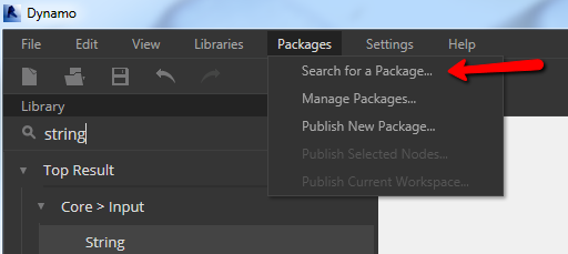
OR:  just get it on the package manager!

Screen Shot 2014-11-21 at 11.22.12 PM

*If for some reason you just want to use this library, but don’t want to use the package manager, you shouldn’t have to worry about building it, check the Pre-Built folder in the github repository and import DynamoUnfold.dll into Dynamo using the import library menu option.

Note : The code is still in a bit of flux. There are a few bugs that crop up with unfolding large models I’m still hunting down.

I welcome forks of this code, discussion, and contributions from others. There are a bunch of places where I know the code is inefficient (converting triangles to surfaces!!, mass intersection of surfaces a polynomial number of times, joining of surfaces into polysurfaces… ), and there are still some really interesting fundamental problems to solve.

State of the Code, an aside

As built at the moment of this writing, this library will attempt to unfold a set of faces, set of surfaces, or a set of surfaces that it will explicitly triangulate, and then unfold the triangular representation. It will not attempt to recognize true developable surfaces like the cone (more below). Instead, to unfold a cone or any curved surface, you must pass the surface geometry of the cone explicitly to UnfoldCurvedSurfacesByTessellation() or Use TessellateSurfaces() to tessellate the surface into a series of triangular surfaces and then pass these to the other surface unfold methods.  You can of course rationalize the surface as you see fit into a set of sub surfaces and pass those to be unfolded, more later.


What This Library Can Do

This library gives you a set of nodes to unfold sets of Faces, Surfaces, or triangulated Surfaces. Faces might come from a solid geometry, surfaces might come from an extrusion or loft.  The three examples below all take some surface geometry as input, tessellate it, and then unfold the resulting tessellation.

There are also nodes for generating labels, before and after the unfold.  The labels are just curve geometry, so they can be generated in Dynamo standalone.

Last, there is a node to pack the resulting unfold parts into a bounding box of the required size.

image

image

image

Some Small Samples

*Note that the structure of this library will probably be changing a bit so that it’s more useable and intuitive.  Some repetitive nodes will be removed and some workflows will be made simpler.  It would be great to get feedback on workflows that users want, but this library does not yet support or are not easy to implement.

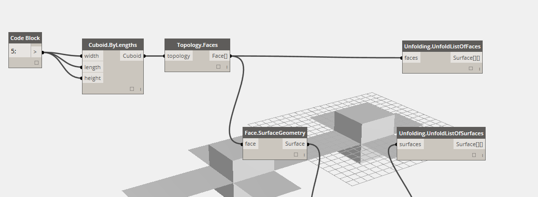
1 .The repo includes a samples folder. The first sample, CubeUnfold, unfolds a cube by surface geometry and faces. The faces are extracted from a solid, and the surfaces are extracted from the faces. Note that there are different nodes for unfolding lists of faces and surfaces.

Screen Shot 2014-09-13 at 5.14.52 PM

2. The second sample, CurvedSurfaceTessellateUnfold,  shows a more complex unfolding operation.

In this sample, we have some curved surface that we tessellate to some level of precision.  The resulting list of surfaces is passed to the unfolding nodes.  We use the UnfoldListOfSurface_AndReturnTransforms node to unfold the list of triangles, and also return the UnfoldingObject - this is a representation of a single unfolding operation, which was performed on a list of surfaces or faces.  The unfolding tracks each surface through the unfold and lets us map things to the final location, like a label.  This means that currently, if you unfold multiple lists of surfaces then each of those lists will generate separate unfolding operations, and the IDs will apply only to that unfolding.  This will come up in the third sample.

After returning the surfaces and unfolding we use the GenerateInitialLabels node to generate some integer IDs and place them on the original surfaces.  Then the GenerateUnfoldedLabels node does what you would expect and places labels with the same ID at the unfolded location.

You can see that the PackUnfoldedSurfaces node requires only the UnfoldingObject as an input, not raw surfaces. This is because the UnfoldingObject stores the surfaces and the transforms through the unfold. This node returns the packed surfaces as well as a new unfolding that lets us label the packed surfaces.

You can see that all label and packing nodes require an unfoldingObject, not raw geometry because we need to keep track of the transformations performed on the surfaces.

Screen Shot 2014-09-13 at 4.37.51 PM

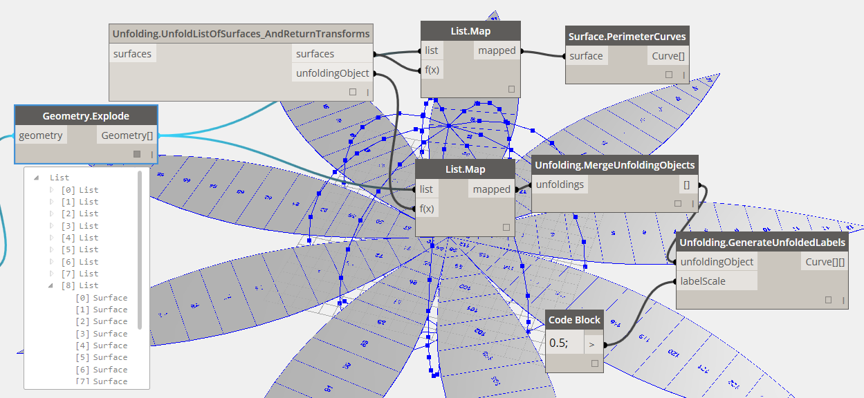
3. The third sample, SphereUnfold, shows a pre-rationalized manual unfolding operation and introduces MergeUnfoldingOperations().

In this sample, the UnfoldListOfSurfaces_AndReturnTransforms node is mapped over a list of nested lists of surfaces. List<List<Surface>>. This mapping returns 9 different UnfoldingObjects, each of which represents an unfolding operation and a list of the associated unfolded surfaces from the surfaces output.

To pack or label these separate unfolding operations all together, we need to merge() them together into one unfolding. This will update all the surface IDs so there are no overlapping IDs, and store all the transformations in one large map. The  MergeUnfoldingOperations() node accepts as input a list of UnfoldingObjects, which is exactly what the second map node returns in the sample.  The final output is one unfolding operation that can be packed or labeled as usual.

This workflow gives you the most flexibility to divide up the unfolding operations into separate jobs you can control and then merge them all back together for labeling and packing.

Screen Shot 2014-09-13 at 12.59.38 PM


Why Unfolding and Unrolling?

image

Image Credit: Walt Disney Concert Hall Logo” by JustefrainOwn work. Licensed under CC BY-SA 3.0 via Wikimedia Commons.

Unfolding and unrolling polyhedra and developable surfaces are related problems. The code discussed in this post deals only with planar faced polyhedra and other solids. To unroll a developable surface with this code we can approximate it by a series of planar faces.

Developable surfaces are a subset of surfaces that can be defined by a series straight ruling lines, along these lines the normal direction at the start and end points are parallel with each other. They have many uses in the context of fabrication because of their properties of constructability.

They can most eaisly be modeled by taking a sheet of paper and twisting it or bending it, without crumpling the paper, all shapes that you are able to make will be defined by a series of straight ruling lines, it stems from the fact that the paper cannot stretch.

Gehry Partners and others make use of the properties of developable surfaces to construct curved surfaces, where in reality, the structural members are straight ruling lines.

The ability to unfold or unroll models is useful for fabrication, model making, and documentation. One can imagine unrolling a complex facade elevation to document it, or even use the unfold as part of the design process, drawing directly onto the unfolded surface, and refolding to see the resulting pattern applied. Once you have an unfolding it’s possible to lasercut, cnc, or handcut the unfolding and put together a model quickly, even for complex shapes. At this point, the code doesn’t handle things like tab generation, but I’ll describe the idea later. The other thing to note is that some unfoldings (even for the same models) will be much easier to construct than others, so we may want to think about metrics for a good unfolding.

Background

Unfolding is a well studied area with lots of interesting open questions. Professor Erik Demaine’s website on folding at: erikdemaine.org has some excellent links to papers, discussions, and code for unfolding.

Approach

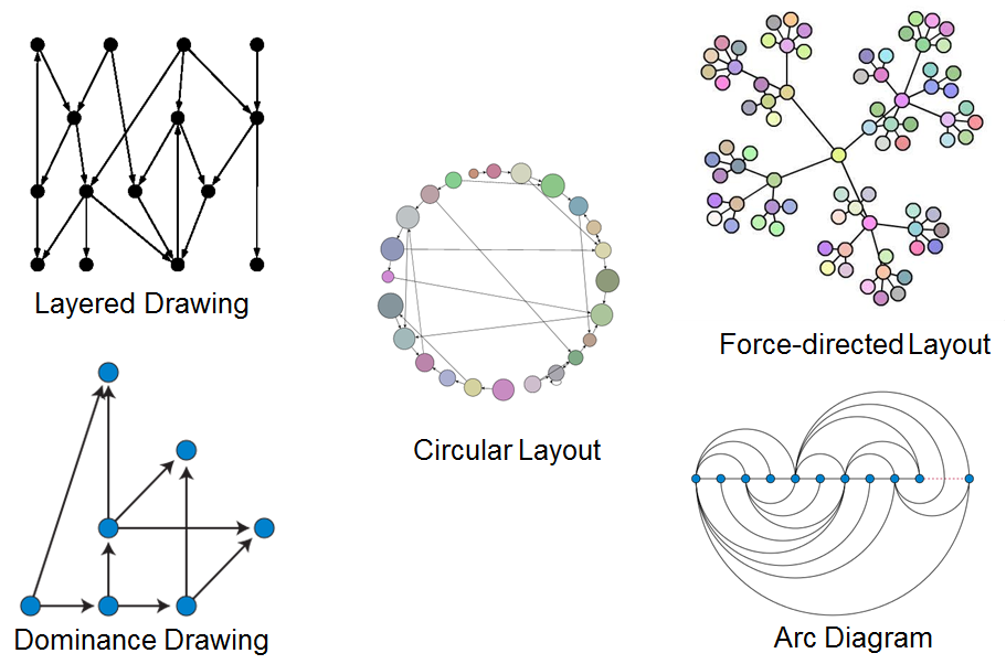
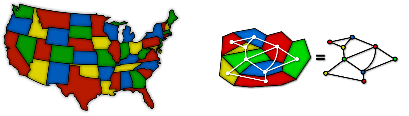
One approach to the unfolding problem is to consider the topology of the object to be unfolded as a graph. In this graph each vertex represents a face in the object, and each edge in the graph represents a coincident edge shared by some number of faces. This graph lets us travel from one face in the object to all adjacent faces, and to reason about these adjacencies. We can build this topology graph by looking at all faces of the model and each edge of that face, if we see an edge twice than we have found a shared edge!
Also graphs are cool.

image

image
-This is the graph that represents a cube, every face is connected to four other faces

In general if we traverse this graph and find a spanning tree, we have found one possible unfolding for the object.

  • A tree is a special kind of graph where there are no cycles, and no vertices that are unreachable.
  • A cycle is a loop.
  • A spanning tree is a tree that includes every vertex from a graph.

So after all that jargon, what we are looking for is a subset of the graph that includes every face but only some edges. These remaining edges are the edges we fold around.

The tree represents not the topology of the object, but the faces, and the edges we will fold them about to produce the unfolding. So finding some spanning tree is the big step that will let us find a possible unfolding.

image

image

- One possible spanning tree of our cube

image

- Another possible spanning tree of a cuboid, this one represents the faces as tessellated triangles so we have 12 faces instead of 6

A spanning tree is not difficult to find for some graph, but the trick is that there are many many many possible spanning trees for most graphs. Most of these will produce different unfoldings. How do we pick which one to actually unfold? A good question. Many of these unfoldings will produce unfolds where the resulting surfaces are overlapping each other. This is not very useful if our purpose is to take the resulting surfaces and cut them out for fabrication. I’ll revisit this question later in this post with some possible solutions.

Algorithm

Once an unfolding tree is found, one can rotate the leaves of the trees to be coplanar with their parents, merging those coplanar faces together and doing this iteratively until all the faces in the tree are coplanar. The leaves of the tree are just the faces in the tree that have no children of their own. The unfolding algorithm is this simple process. The rotation is done two graph vertices at a time, and as the faces become merged together we rotate those merged faces as if they were one. At each step we must calculate the angle between two surfaces, the child and its parent.

image

image

Explicity The steps are:

  • find a leaf in the tree – this is a face we’ll fold, that has no folds after it, call this the child
  • find this face’s parent – the parent represents the face we need to make the child coplanar with.
  • find the edge that points from the parent face to the child, this edge represents the edge we’ll rotated around, the fold edge.
  • rotate the child to be coplanar with the parent.
  • check if this rotation caused any overlaps to occur with previously unfolded faces.
  • if not, then join the parent and child surface into a polysurface and store this polysurface in the tree node that used to represent the parent face.
  • remove the child node from the tree – this is a contraction of the parent and child nodes into one node.
  • repeat until there is only one node left in the tree.

This process outlined above is almost the entire story. There’s a bit more that happens if there is an overlap.

Dealing with Overlaps During The Unfold

If during the algorithm outlined above, the rotation of the current surface to be coplanar with its parent, causes an overlap of a previously unfolded face with the current face, we need to do something. A simple solution is to move the current surface away from the rest of the unfold. It’s either a single surface or some chain of already coplanar surfaces, so it’s safe to stop unfolding it and put it somewhere else. We can make it planar with the rest of the unfolding at the very end. Problem solved …Well…Kinda…

What’s the worst case? That every time we rotate a face up to be coplanar with its parent we end up with an overlap, then we wont have a nice unfolding, but just a bunch of separate faces, still useful, but not great.

As I mentioned before, this hypothetical unfolding that is causing all these overlaps is not the only unfolding for this hypothetical model. There exists many more unfoldings we could try. At this time, this idea is unimplemented, but one could think of this problem as an optimization or search problem, minimizing or searching for a small number of subparts for the unfold. You would need some way to generate a random unfolding tree, a way to modify that unfolding tree, and a way to evaluate the final unfolding.

This should lead you ask the question, what if there is no good unfolding for a particular model? Well that is one of those interesting open questions surrounding the study of unfoldings. Does there exist a simple (non-overlapping) unfolding for every polytope? So, since that’s an open question, we need some way of stopping this search if we can’t find one fast enough. Iterating all possible spanning trees could take… a while. It’s difficult to define the number of spanning trees in terms of verts and edegs of a graph, but it is almost certainly too many to brute force through in the time we would like in Dynamo.

Simple Implementation

To find some spanning tree I’m currently using an implementation of Breadth First Search. It’s fast and simple. It gives us two nice attributes when it’s finished. A tree, and a distance associated with each node in the tree. This lets us quickly find the leaves of tree, since the highest distances will be the leaves, so we can sort the tree by the distance of each node. Keep in mind BFS only produces one possible unfolding, and it could be one with many overlaps, even if a simple unfolding exists.

image

- The spanning tree generated from this developable surface represented as a series of triangles – the spheres represent each face, the edges represent the shared edges, but note these are edges in the tree, not geometrical edges!, also this tree is really easy to unfold, it’s a linked list! AND it’s also a Hamiltonian Path – it’s guaranteed to have a simple unfolding

So Many Surfaces! – Dynamo’s Geometry Library

Interacting with Protogeometry through C#, Dynamo’s wrapper for Autodesk Shape Manager is fairly simple in most cases. The methods are the same ones that are exposed in Dynamo as nodes, so they should be pretty familiar.

Creating Geometry

The first thing to note, is that like the methods exposed in Dynamo, to create new geometry we don’t use the new keyword, we use static constructors in the class of the geometry like in Dynamo or DesignScript.

var myNewPoint = Point.ByCoordinates(0,0,0);

Another important aspect of the library is that these geometrical entities are mostly immutable. When you perform any kind of geometrical transformation you are producing new geometry. This is great, and causes some headaches as well.

var anotherNewerPoint = myNewPoint.Translate(1,0,0);

Some Headaches

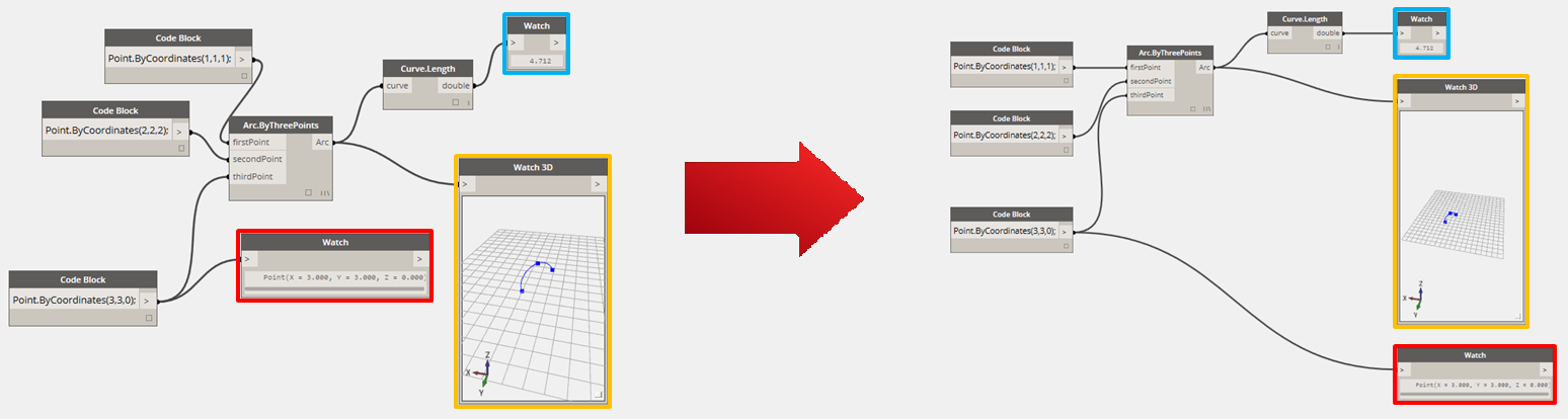
The headaches with immutable geometry arise when you want to tag some instance of geometry with some information. For example, we want to tag a specific face in our unfolding with a label. It would be nice to be able to tag this face before running the unfolding algorithm, and when the unfolding is finished, iterate each face and grab the label and display it. We can’t do this, since the final faces of the unfold are all brand new surfaces, and won’t contain any information we tag them with.

The solution that I use in this code is to build a map of transformations to geometry that tracks all the transformations that apply to a set of surfaces. For the label example, we can now iterate the original faces, lookup the label we associated with the original face and then lookup the transformations that apply to this face throughout the unfold. Then just apply all the transformations to that label, and it will move to the final position, as if it had been associated with the face.

Actually moving this information through the unfolding is a bit trickier, but it’s very similar to merging the parent and child surfaces together and storing them in the parent surface. At each step of the unfold we want to record the new coordinate system of the rotated faces, and which faces were actually rotated.

Working With Zero Touch and Protogeometry.

Create Your Own Nodes

Skip to Zero Touch Directly

For some issues with running unit tests for zero touch nodes on top of protogeometry check the readme on DynamoUnfold. The short version is that Dynamo uses host applications on your machine to drive its geometry engine, and to test a standalone project that uses the geometry engine, we’ll need to reference some of those applications as well. The state of this interop should become much simpler in the future, for now it’s just a bit of work to get testing. (In fact, that work is being done on the zero touch samples right now by Ian himself.)

I hope you enjoyed this blog post, I plan to continue refining the repository and cleaning up the build process and functionality. Have fun.
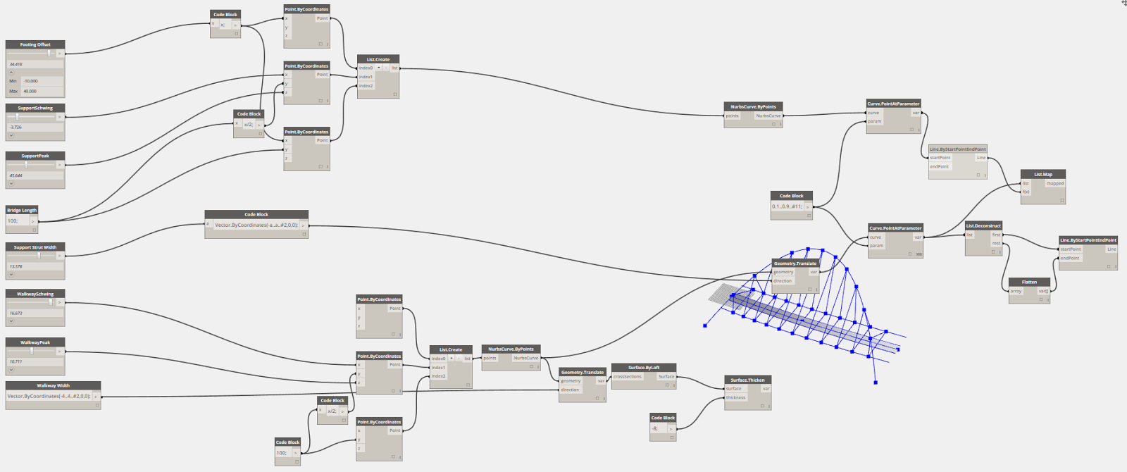
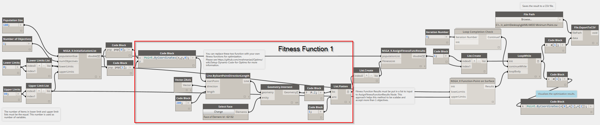
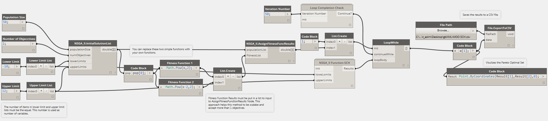
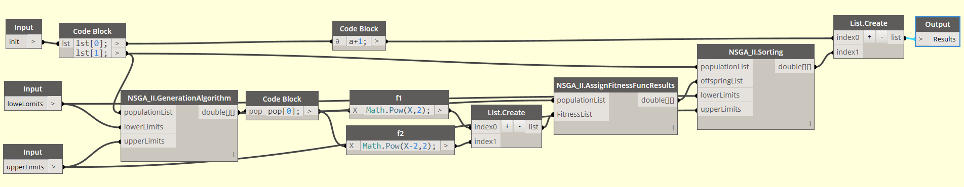
 

Dynamo 0.7.4 Release

$
0
0

Welcome to the next incremental improvement to all things Dynamo.  We’ve been getting ready for Autodesk University and trying to make sure folks who are building out additional functionality are happy, as well as doing general bug fixing and a couple of target improvements.  Also don’t forget to check out some of the excellent emerging extensions to Dynamo functionality that have come out, like Optimo and Unfolding, and watch the Package Manager for new additions all the time.

Check out the ReadMe for a more complete list, and see the list of know issues at the bottom of this post, but here are a couple of specific things to look for.

Reading files from Disk:

In 0.7.3 and before, Dynamo only read files from disk once, then would not check the file again for any changes.  Files that Dynamo was accessing would also lock them, making it difficult or impossible to edit them while Dynamo was on.  In Dynamo 0.7.4, we have the ability to monitor files on disk for changes and update the Dynamo graph when it does, and Dynamo does not lock up files being read, allowing for live editing and update.  To take advantage of this, it is necessary to make a small change to existing definitions.  Read nodes used to take a file path (a string) and will now take a file object.  For instance, if you were reading data from an Excel file in 0.7.3, you would have this:

Now, Excel and other Reader nodes will require an intermediate step to watch the data coming in.

Old workflows to still migrate up to 0.7.4 with a small warning indicating that users should make this adjustment to their workflows. The old nodes will have the same static behavior as before.

Structural Framing:

We have made the creation of structural framing elements much easier.  Placing structural framing in  0.7.3 required users grappling with 5 input types, at least 2 of which were non-sensical to non-programmers and one that didn’t work (UpVector, at least in an obvious way).  We are preserving the old node, as there are some edge cases where it still makes sense to use have it available, but we are breaking this functionality out into 3 more specific nodes, creating Beams, Braces, and Columns, with only 3 needed inputs.

In order to rotate the framing member, which seems like “up vector” should (but doesn’t in most cases) address, users can manipulate the “Cross-Section Rotation” parameter that is a built-in parameter for every member.

A couple other things we hope you have had a chance to take a look at:

Package Manager Improvements:  some UI enhancements and, for folks who are distributing and consuming libraries (like DynaWorks15 or others), only the specified nodal functionality is shown (ancillary libraries were being surfaced before, which could clutter your search/browse capabilities).

Datasets distributed via the Package Manager:

This was already in 0.7.3, but we want to call it out again, as it allows you to push out new content to your users to illustrate ideas or use base dyn files or rvt files, or pretty much anything.  We’re hoping this becomes a useful teaching tool, look for these additional datasets by browsing to %AppData%\Roaming\Dynamo\0.7\packages

Known issues we are working on:

- Element.Geometry may cause a crash in Dynamo versions 0.7.2-0.7.4 when run in Revit 2015 when executed on large groups of Revit geometry.

- Upgraded Excel.Write nodes will show as “Unresolved”.  They can be replaced with Excel.Write to File nodes.

- View.ExportAsImage will only export {3d}

- Cancel does not work when executing Cloud based Renderings, this includes Daylighting.

- Dynamo can fail to launch in Revit when Unifi,  Maxwell, or Kiwi Bonus Tools add-in is installed on Revit 2015.  If you have one of these applications installed, or find that Dynamo fails to launch from the addins menu, this is fixed in the latest Pre-Release Builds.

- Existing Code Block Nodes may be affected by name collisions with functions that come from installed packages.  For instance, Point.ByCoordinates is affected by a collision with a Point. operation in the popular Rhynamo package and will throw an error saying “Warning: Dereferencing a non-pointer. Dereferencing a non-pointer.” To correct this, re-enter the function in the code block node, autocorrect will indicate a more specific refererence.


Great Speakers at the AU Design Computation Symposium 2014

$
0
0

Don’t forget to sign up for the Design Computation Symposium this year at Autodesk University 2014. Register for this session.

December 3, 2014 | 8:00 am – 12:00 pm
Mandalay Bay F, Level 2 | Mandalay Bay Hotel, Las Vegas, Nevada

We have an amazing lineup of speakers this year:


Session 1: 08:00 am – 09:30 am
08:00 am – 08:05 am Introductions Matt Jezyk
08:05 am – 08:15 am Craftsmanship and Digital Fabrication, Pier 9 Carl Bass
08:15 am – 08:45 am Hy-Fi David Benjamin
08:45 am – 09:30 am Keynote 1: Reshaping Urban Airspace Janet Echelman
09:30 am – 10:00 am Break  
 
Session 2: 10:00 am – 12:00 pm
10:00 am – 10:30 am Designing a New Materialism Andy Payne
10:30 am – 11:00 am Unlocking Robotic Design Sigrid Brell-Cokcan
11:00 am – 11:45 am Keynote 2: Craft, digital fabrication, and digital assembly Mark Burry
11:45 am – 12:00 pm Closing Remarks, Q&A  


Interested? Sign up here


More information on our great speakers:

David-Benjamin-Photo

David Benjamin is Founding Principal of The Living and Assistant Professor at Columbia University Graduate School of Architecture, Planning and Preservation. The Living brings new technologies to life in the built environment, integrating design innovation, sustainability, and the public realm. Clients include the City of New York, 3M, Airbus, and Miami Science Museum. Recent projects include the Princeton Architecture Laboratory (a new building for research on next-generation design and construction technologies), Pier 35 EcoPark (a 200-foot floating pier in the East River that changes color according to water quality), and Hy-Fi (a branching tower for the Museum of Modern Art and MoMA PS1 made of a new type of biodegradable brick). The Living was recently acquired by Autodesk.


Andrew Payne_Headshot

Andrew Payne is an architect and Senior Building Information Specialist at Case-Inc. He recently completed his Doctoral degree at Harvard’s Graduate School of Design where his dissertation examined new personalized intelligent comfort control strategies for office spaces.  Andrew’s other research interests focus on embedded computation, parametric design, robotics, microcontrollers, and 3d printing.  He is the co-author (with Jason K. Johnson) and lead developer of Firefly – a software plugin which bridges the gap between the digital CAD environment of Rhino/Grasshopper (and soon to be Dynamo) with physical input/output devices like the Arduino, web cams, mobile phones, game controllers and more.  He has lectured and taught workshops throughout the United States, Canada, and Europe and has held teaching positions at Columbia University and the Pratt Institute.  He also sits on the Board of Directors for the Association for Computer Aided Design in Architecture (ACADIA).


Brell-Cokcan

Co-founded by Sigrid Brell-Cokcan and Johannes Braumann in 2010 the Association for Robots in Architecture has been pioneering the easy use of industrial robots for the creative industry. They are participating in international research and industry projects and have recently become KUKA System partners and a validated EU research institution under the FP7 program.

Sigrid Brell-Cokcan is a professional architect with her own successful architecture firm II Architects int in Istanbul and Vienna and is currently holding the first international professorship for “creative robotics” at the industrial design department of the University for Art and Industrial Design, Linz/ Austria.


JanetEchelman_PhotoToddErickson_GEP_9703b

American artist Janet Echelman builds soft, billowing sculpture at the scale of buildings that respond to the forces of nature – wind, water, and light. She combines ancient craft with custom Autodesk technology to create ultra-lightweight sculptures that move gently with the wind in ever-changing patterns. Her recent sculpture Skies Painted with Unnumbered Sparks, a 745-ft sculpture that premiered at the 2014 TED Conference, the largest pre-stressed rope structure in the world. She recently received the 2014 Smithsonian Ingenuity Award in Visual Arts, honoring “the greatest innovators in America today.”


Mark Burry 04JUNE10JM-99

Professor Mark Burry is a practising architect who has published internationally on two main themes: the life, work and theories of the architect Antoni Gaudí, and putting theory into practice with regard to ‘challenging’ architecture. He has been Senior Architect to the Sagrada Família Basilica Foundation since 1979 pioneering distant collaboration with his colleagues based on-site in Barcelona.  He is currently the Founding Director of the RMIT University’s Design Research Institute (DRI), established in 2008 to collaborate across the entire university design community ranging from hard-core sciences and technology to applied arts. In 2001 he founded RMIT University’s state-of-the-art Spatial Information Architecture Laboratory (SIAL) in Melbourne Australia, established as a holistic transdisciplinary spatial design research environment.

0..4 Tips and Tricks

$
0
0

In honor of Autodesk University 2014 this week—with hundreds of people learning Dynamo in Las Vegas—I’d like to share some tips that will help you get more out of your Dynamo. Stay tuned for more in the series.

[0] Hot Keys

[0] Use F5 to Run the graph… I know. Epic.
F5ToRun
[1] Hold down ESC to navigate the background geometry preview or use CTRL + G to toggle between geometry and node modes. I personally think ESC is a lot faster to use.
[2] Hit ESC once to clear text from the library search box.
[3] The usual suspects:
[0] CTRL + C to copy nodes or text.
[1] CTRL + N to create a new file.
[2] CTRL + O to open an existing file.
[3] CTRL + S to save, CTRL + Shift + S to save as.
[4] CTRL + V to paste nodes or text.
[5] CTRL + X to cut nodes or text.
[6] CTRL + Y to redo.
[7] CTRL + Z to undo.
[4] Use CTRL + L to automatically arrange your nodes.
[5] Use CTRL + W to make a note.
note
[6] Show or hide the console with CTRL + Shift + ⇧ (or just drag the top edge up or down with your mouse).

[1] Make Lists

[0] Use Number Sequence and Number Range.

ranges

[1] Use range syntax. Now do you get the title?! (From Dynamo, see Help/Samples/Core/CoreRangeSyntax.)

ranges2

[2] Use List.Create. Use a series of these to create nested lists.

lists4

[3] Use List.Join. This node, different from List.Create, flattens any hierarchy in the resultant list.

lists5

[4] Use { } in a code block. Remember to include the ; at the end of the line. Nested braces create nested lists.

lists6

[2] Access List Items

[0] In Dynamo, like in most other programming languages, lists are zero-indexed. So the first item is #0, and the last item is #(total_number_of_items – 1).
fingers
[1] Use the node List.GetItemAtIndex.

lists1

[2] Use a range expression to get multiple items.

lists2

[3] Use [ ] in a code block.

lists3

[3] Node Options

[0] Right-click to toggle the geometry preview on or off. (starShape.dyn)

preview

[1] Right-click to show the list indices for previewed geometry. (circlePacking.dyn)

showLabels

[4] Auto-Complete

[0] Double-click in the canvas to get a code block. You can call nodes by typing their names here instead of using the node itself. See this post for more.
[1] Auto-complete in a code block helps you discover functionality in the library and to avoid misspellings. Press Enter to accept or ESC to ignore the suggestions.

autocomplete1

[2] Use a dot (just like in the node name) to browse which methods are available to use for the class.

autocomplete2

[3] See the different “overrides” for a method name. This is a guide for which inputs to use and in what order.

autocomplete3

AU2014 Design Computation Symposium Recording Online Now

$
0
0

If you attended the Design Computation Symposium  last week you were fortunate enough to see some of the most captivating speakers at at AU2014 conference. This year the entire session was recorded and is now available online. Check it out!

AU2014DesignCompSpeakers

Autodesk CEO Carl Bass kicked off the event speaking about his personal creative work and how that intersects with digital fabrication. David Benjamin explained the design and fabrication process behind the Hy-Fi installation at New York MoMa PS1 and then Janet Echelman went in depth into the design process her studio uses to make amazing hanging net sculptures.  After a short break Andy Payne blew our minds with his work from the Harvard GSD on multi-material 3d printing and a new application he and other GSD colleagues are creating called Monolith, a new voxel-based 3d design and fabrication tool. Sigrid Brell-Cocken amazed us with the work she is doing at Robots In Architecture, maybe we call her the “robot whisperer’ now!. And then, of course, to bring the event home we were very pleased to have Mark Burry give us the definitive history of Design Computation, geometry and fabrication techniques, all wrapped up in his amazing work on Gaudi’s Sagrada Família.     I would like to thank our list of speakers once again and invite you to watch the recording online.

Session 1: 08:00 am – 09:30 am
Craftsmanship and Digital Fabrication  Carl Bass
Hy-Fi   David Benjamin
Reshaping Urban Airspace   Janet Echelman
Session 2: 10:00 am – 12:00 pm
Designing a New Materialism   Andy Payne
Unlocking Robotic Design   Sigrid Brell-Cokcan
Craft, digital fabrication, and digital assembly   Mark Burry

More information on the speakers: http://dynamobim.com/great-speakers-at-the-au-design-computation-symposium-2014/ 

1st Annual Dynamo Hackathon

$
0
0

At this year’s Autodesk University, four teams participated in the first annual Dynamo Hackathon, developing new tools, hacks, experiments, and workflows using Dynamo. We’d like your help choosing a winner. Please take a moment to look at this work and vote for your favorite.


Document Elements Location By Coordinates in Revit

Eric Boehlke

2

4

5

Project Website


Animate design iterations in Revit with Dynamo

Andreas Dieckmann, Havard Vasshaug, Julien Benoit, Ian Siegel

Screen Shot 2014-12-15 at 11.37.45 AM

Screen Shot 2014-12-15 at 11.38.28 AM

Read more here.


Drawing with Dynamo

Patrick Tierney & David Thomasson

IMG_3712


Designed by the Sound

Andrea Vannini & Michael Hudson

Screen Shot 2014-12-15 at 11.55.12 AM

Screen Shot 2014-12-15 at 11.55.49 AM


Vote Here

White Christmas with Dynamo

$
0
0

A big thanks to Colin who helped review this article and made it human readable!

There are designers, and then there is everyone else. I am most definitely not a designer, but then again, Dynamo was not built for just designers—it was built for users and for uses that we knew we couldn’t fully anticipate. Dynamo is an extremely flexible system, and with each new feature introduction comes new possibilities. This write-up represents my experiment with one such new functionality in Dynamo: periodic evaluation (we are finalizing the design, soon as all the details are ironed out, this new feature will be enabled in the daily build).

What better way to wish you Happy Holidays (and to test out my project) than to make Dynamo sing to you?!

Getting the Data

A MIDI file (short for “Musical Instrument Digital Interface”) contains information including tracks with MIDI commands. These commands are sent to a speaker during playback, resulting in the music that we hear.

In order to pass these MIDI commands through Dynamo to a MIDI output device, we must first have a way to load them into a Dynamo graph. For this exercise, I chose to use Microsoft Excel. Why not, right?

This is where the C# MIDI Toolkit comes in handy. This open source toolkit is capable of loading any MIDI file. With a few tweaks, I was able to write track information (MIDI commands) out to a CSV format. Each command is written out to the CSV file in a tick-command value pair, with each tick, in milliseconds, marking the absolute time at which a MIDI command should be sent to the output. This process results in two Excel worksheets, one for each of the two tracks in the MIDI file I used. (Column headers are added for illustration only.)

excel-white-christmas-track

The following partial Dynamo graph imports one of these Excel worksheets into Dynamo. The File.FromPath node converts the file path, which is just a string, into a file object to be “watched” by Dynamo for changes. Then I chose the sheet name, called “Track0″, and I read the data with Excel.ReadFromFile. Then List.Transpose is used to flip row-oriented data into column-oriented data for downstream consumption (we would like to have ticks and commands in separate lists).

Reading Excel file with Excel node

Tempo and Playback Speed

The playback speed of a MIDI file is determined by both its tempo and time division values.

Tempo is measured in microseconds per quarter note. This value is specified by “Set Tempo” meta-event (an event that is not sent or received over a MIDI port), and in our case it has a value of 600,000. This means a quarter note lasts 600,000 microseconds or 600 milliseconds.

The time division is measured in pulses per quarter note (PPQN), which specifies the number of ticks that correspond to a quarter note. For the MIDI file in this experiment, we will use 192 ticks per quarter note.

With these two pieces of information, it is possible to translate an absolute tick value for any given MIDI command into real world time. Consider the following highlighted MIDI command and its absolute tick value:

MIDI Commands vs. Ticks

The MIDI command in the second column should be sent when the absolute tick count reaches 384. Given that a quarter note = 192 ticks and lasts for 600 milliseconds, the command should be sent just as 384 ticks = 2 quarter notes = 1200 milliseconds has elapsed. Or, more generally, in case you like to see the math:

Time Conversion  Equation

Next in the Dynamo graph, the absolute tick values imported from the Excel worksheet are translated into milliseconds since the playback is based on real world time. The following graph shows how:

Time Conversion

MIDI Playback

We do not need more than a very primitive way to render our MIDI data for this experiment—all we need is a handful of Win32 API calls and minimal time management code around them, and voila! We have a bare-bones MIDI player. The following sections describe these classes. (Feel free to skip ahead if you so choose!)

Track Class

This class serves as a container for the actual data for a single MIDI track. A node of this type is constructed by taking two input arrays of the same size: time values in milliseconds and MIDI commands.

public class Track
{
    private readonly List milliseconds;
    private readonly List commands;

    private Track(IEnumerable milliseconds, IEnumerable commands)
    {
        this.milliseconds = new List(milliseconds);
        this.commands = new List(commands);
    }

    public static Track FromTrackData(
        double[] milliseconds, double[] commands)
    {
        return new Track(milliseconds, commands);
    }

    internal void FetchCommands(double millisecond, ICollection fetched)
    {
        while (milliseconds.Count > 0)
        {
            if (milliseconds[0] >= millisecond)
                break;

            fetched.Add(commands[0]);
            milliseconds.RemoveAt(0);
            commands.RemoveAt(0);
        }
    }
}

Timer Class

A time management class keeps track of the current elapsed time in milliseconds. Its sole purpose is to increment the time by a specific amount each time its Tick method is called. The Timer class provides a single reference of time that is tolerant to delays between consecutive evaluations. For example, if the first call to Tick takes longer than the desirable duration to finish, the second call to Tick will only increase the time by an amount appropriate to maintaining overall regularity.

public class Timer
{
    private double currentMilliseconds;
    private readonly double incrementInMs;

    private Timer(double incrementInMs)
    {
        this.incrementInMs = incrementInMs;
    }

    public static Timer FromIncrement(double milliseconds)
    {
        return new Timer(milliseconds);
    }

    public double Tick()
    {
        currentMilliseconds += incrementInMs;
        return currentMilliseconds;
    }
}

Sequencer Class

A node of this type is constructed by an array of input Track nodes. Its main purpose is to retrieve MIDI commands from Track objects and feed them through to Win32 APIs for MIDI playback.

public class Sequencer : IDisposable
{
    #region Win32 Midi Output Functions and Constants

    [DllImport("winmm.dll")]
    private static extern int midiOutOpen(ref int handle, int deviceID,
        MidiOutProc proc, int instance, int flags);

    [DllImport("winmm.dll")]
    private static extern int midiOutClose(int handle);

    [DllImport("winmm.dll")]
    protected static extern int midiOutShortMsg(int handle, int message);

    protected delegate void MidiOutProc(int handle,
        int msg, int instance, int param1, int param2);

    #endregion

    private int deviceId;
    private int deviceHandle;
    private const int CALLBACK_FUNCTION = 196608;

    private readonly Track[] tracks;

    private Sequencer(Track[] tracks)
    {
        this.tracks = tracks;

        midiOutOpen(ref deviceHandle, deviceId,
            HandleMessage, 0, CALLBACK_FUNCTION);
    }

    public static Sequencer FromTracks(Track[] tracks)
    {
        return new Sequencer(tracks);
    }

    public void Dispose()
    {
        if (deviceHandle != 0)
        {
            midiOutClose(deviceHandle);
            deviceHandle = 0;
        }
    }

    public Sequencer ProcessTick(double milliseconds)
    {
        if (deviceHandle == 0)
            return this;

        var commands = new List();
        foreach (var track in tracks)
            track.FetchCommands(milliseconds, commands);

        foreach (var command in commands)
        {
            var message = ((int) command);
            midiOutShortMsg(deviceHandle, message);
        }

        return this;
    }

    private void HandleMessage(int handle, int msg,
        int instance, int param1, int param2)
    {
    }
}

Challenges

Managing something as time-sensitive as playing a MIDI file is a challenge. Dynamo’s scheduler thread in which evaluations take place is not of real-time priority and can be affected by various external factors. Just one example, the screen recording software I used for the demo video affects MIDI playback slightly whenever it writes to disk.

Even without external factors, graph evaluation is not guaranteed to complete within an acceptable interval before the next batch of MIDI commands must be sent, causing hiccups during playback.

Luckily for the sample MIDI file though, the gap between MIDI command batches averages around 300 milliseconds (although a few commands have start time that is slightly off from an even multiple of 300 milliseconds), and the gaps are too small to notice. So if we really wanted to, we could set the graph-wide evaluation period to be 300 milliseconds and still maintain a reasonable playback result.

Putting It All Together

In order to periodically send MIDI commands to the output device, the graph needs to be reevaluated at a fixed interval of 300 milliseconds. The only two nodes that must be reevaluated are Timer.Tick and Sequencer.ProcessTick. The following image illustrates the way to mark both the nodes as requiring update whenever the periodic evaluation kicks in.

Dynamo Periodic Update Context Menu

This is the completed graph for the experiment (click to enlarge):

Complete graph for MIDI playback in Dynamo

Video Demo

The video below demonstrates the whole workflow (see the HD version on YouTube for better visual quality):


Happy holidays!

With that, I wish everyone in Dynamo community and my fellow teammates a Merry Christmas and a happy new year!

Viewing all 41 articles
Browse latest View live


<script src="https://jsc.adskeeper.com/r/s/rssing.com.1596347.js" async> </script>